Pre-Class Reading and Video
Thus far, we have focused on descriptive statistics. Through our examination of frequency distributions, graphical representations of our variables, and calculations of center and spread, the goal has been to describe and summarize data. Now you will be introduced to inferential statistics. In addition to describing data, inferential statistics allow us to directly test our hypothesis by evaluating (based on a sample) our research question with the goal of generalizing the results to the larger population from which the sample was drawn.
Hypothesis testing is one of the most important inferential tools of application of statistics to real life problems. It is used when we need to make decisions concerning populations on the basis of only sample information. A variety of statistical tests are used to arrive at these decisions (e.g. Analysis of Variance, Chi-Square Test of Independence, etc.). Steps involved in hypothesis testing include specifying the null (H0) and alternate (Ha or H1) hypotheses; choosing a sample; assessing the evidence; and making conclusions.
Statistical hypothesis testing is defined as assessing evidence provided by the data in favor of or against each hypothesis about the population.
Please watch the video below on the fundamentals involved in hypothesis testing:
Example:
To test what I have read in the scientific literature, I decide to evaluate whether or not there is a difference in smoking quantity (i.e. number of cigarettes smoked) according to whether or not an individual has a diagnosis of major depression.
Let’s analyze this example using the 4 steps: Specifying the null (H0) and alternate (Ha) hypotheses; choosing a sample; assessing the evidence; and making conclusions.
There are two opposing hypotheses for this question:
- There is no difference in smoking quantity between people with and without depression.
- There is a difference in smoking quantity between people with and without depression.
The first hypothesis (aka null hypothesis) basically says nothing special is going on between smoking and depression. In other words, that they are unrelated to one another. The second hypothesis (aka the alternate hypothesis) says that there is a relationship and allows that the difference in smoking between those individuals with and without depression could be in either direction (i.e. individuals with depression may smoke more than individuals without depression or they may smoke less).
1. Choosing a Sample:
I chose the NESARC, a representative sample of 43,093 non-institutionalized adults in the U.S. As I am interested in evaluating these hypotheses only among individuals who are smokers and who are younger (rather than older) adults, I subset the NESARC data to individuals that are 1) current daily smokers (i.e. smoked in the past year CHECK321 ==1, smoked over 100 cigarettes S3AQ1A ==1, typically smoked every day S3AQ3B1 == 1) are 2) between the ages 18 and 25. This sample (n=1320) showed the following:
- Young adult, daily smokers with depression smoked an average of 13.9 cigarettes per day (SD = 9.2).
- Young adult, daily smokers without depression smoked an average of 13.2 cigarettes per day (SD = 8.5).
While it is true that 13.9 cigarettes per day are more than 13.2 cigarettes per day, it is not at all clear that this is a large enough difference to reject the null hypothesis.
2. Assessing the Evidence:
In order to assess whether the data provide strong enough evidence against the null hypothesis (i.e. against the claim that there is no relationship between smoking and depression), we need to ask ourselves: How surprising is it to get a difference of 0.7373626 cigarettes smoked per day between our two groups (depression vs. no depression) assuming that the null hypothesis is true (i.e. there is no relationship between smoking and depression).
This is the step where we calculate how likely it is to get data like that observed when H0 is true. In a sense, this is the heart of the process, since we draw our conclusions based on this probability.
It turns out that the probability that we’ll get a difference of this size in the mean number of cigarettes smoked in a random sample of 1320 participants is 0.1711689 (do not worry about how this was calculated at this point).
Well, we found that if the null hypothesis were true (i.e. there is no association) there is a probability of 0.1711689 of observing data like that observed.
Now you have to decide…
Do you think that a probability of 0.1711689 makes our data rare enough (surprising enough) under the null hypothesis so that the fact that we did observe it is enough evidence to reject the null hypothesis?
Or do you feel that a probability of 0.1711689 means that data like we observed are not very likely when the null hypothesis is true (not unlikely enough to conclude that getting such data is sufficient evidence to reject the null hypothesis).
Basically, this is your decision. However, it would be nice to have some kind of guideline about what is generally considered surprising enough.
The reason for using an inferential test is to get a p-value. The p-value determines whether or not we reject the null hypothesis. The p-value provides an estimate of how often we would get the obtained result by chance if in fact the null hypothesis were true. In statistics, a result is called statistically significant if it is unlikely to have occurred by chance alone. If the p-value is small (i.e. less than 0.05), this suggests that it is likely (more than 95% likely) that the association of interest would be present following repeated samples drawn from the population (aka a sampling distribution).
If this probability is very small, then that means that it would be very surprising to get data like that observed if the null hypothesis were true. The fact that we did not observe such data is therefore evidence supporting the null hypothesis, and we should accept it. On the other hand, if this probability were very small, this means that observing data like that observed is surprising if the null hypothesis were true, so the fact that we observed such data provides evidence against the null hypothesis (i.e. suggests that there is an association between smoking and depression). This crucial probability, therefore, has a special name. It is called the p-value of the test.
In our examples, the p-value was given to you (and you were reassured that you didn’t need to worry about how these were derived):
- P-Value = 0.1711689
Obviously, the smaller the p-value, the more surprising it is to get data like ours when the null hypothesis is true, and therefore the stronger the evidence the data provide against the null. Looking at the p-value in our example we see that there is not adequate evidence to reject the null hypothesis. In other words, we fail to reject the null hypothesis that there is no association between smoking and depression.
Since our conclusion is based on how small the p-value is, or in other words, how surprising our data are when the null hypothesis (H0) is true, it would be nice to have some kind of guideline or cutoff that will help determine how small the p-value must be, or how “rare” (unlikely) our data must be when H0 is true, for us to conclude that we have enough evidence to reject H0. This cutoff exists, and because it is so important, it has a special name. It is called the significance level of the test and is usually denoted by the Greek letter α. The most commonly used significance level is α=0.05 (or 5%). This means that:
- if the p-value <α (usually 0.05), then the data we got is considered to be “rare (or surprising) enough” when H0 is true, and we say that the data provide significant evidence against H0, so we reject H0 and accept Ha.
- if the p-value >α (usually 0.05), then our data are not considered to be “surprising enough” when H0 is true, and we say that our data do not provide enough evidence to reject H0(or, equivalently, that the data do not provide enough evidence to accept Ha).
Although you will always be interpreting the p-value for a statistical test, the specific statistical test that you will use to evaluate your hypotheses depends on the type of explanatory and response variables that you have.
Bivariate Statistical Tools:
- C→Q: Analysis of Variance (ANOVA)
- C→C: Chi-Square Test of Independence (χ2)
- Q→Q: Correlation Coefficient (r)
- Q→C: Logistic regression
A sampling distribution is a distribution of all possible samples (of a given size) that could be drawn from the population. If you have a sampling distribution meant to estimate a mean (e.g. the average number of cigarettes smoked in a population), this would be represented as a distribution of frequencies of mean number of cigarettes for consecutive samples drawn from the population. Although we ultimately rely on only one sample, if that sample is representative of the larger population, inferential statistical tests allow us to estimate (with different levels of certainty) a mean (or other parameter such as a standard deviation, proportion, etc.) for the entire population. This idea is the foundation for each of the inferential tools that you will be using this semester.
Confidence Intervals
(This section is adapted from the United States Census Bureau)
Another inferential tool is confidence intervals. They give us more detailed information than hypothesis tests, but allow us to answer similar types of questions.
What is a confidence interval?
A confidence interval is a range of values that describes the uncertainty surrounding an estimate. We describe a confidence interval by its endpoints; for instance, the 95% confidence interval for the proportion of people who think the Supreme Court is doing a good job is “0.409 to 0.471”. A confidence interval is also itself an estimate. It is made using a model of how sampling, interviewing, measuring, and modeling contribute to uncertainty about the relation between the true value of the quantity we are estimating and our estimate of that value.
How do we interpret a confidence interval?
The “95%” in the confidence interval listed above represents a level of certainty about our estimate. If we were to repeatedly make new estimates using exactly the same procedure (by drawing a new sample, conducting new interviews, calculating new estimates and new confidence intervals), the confidence intervals would contain the average of all the estimates 95% of the time. We have therefore produced a single estimate in a way that, if repeated indefinitely, would result in 95% of the confidence intervals formed containing the true value.
We can increase the expression of confidence in our estimate by widening the confidence interval. For the same estimate, the 99% confidence interval is wider — “0.399 to 0.481”. Different disciplines tend to select different levels of confidence. 95% confidence intervals are the ones we typically use for this course (and are generally the most common).
Why have confidence intervals?
Confidence intervals are one way to represent how “good” an estimate is; the larger a 95% confidence interval for a particular estimate, the more caution is required when using the estimate. Confidence intervals are an important reminder of the limitations of the estimates.
ANOVA
In our description of hypothesis testing in the previous chapter, we started with case C→Q, where the explanatory variable/independent variable/predictor (X = major depression) is categorical and the response variable/dependent variable/outcome (Y = number of cigarettes smoked) is quantitative. Here is a similar example:
GPA and Year in College
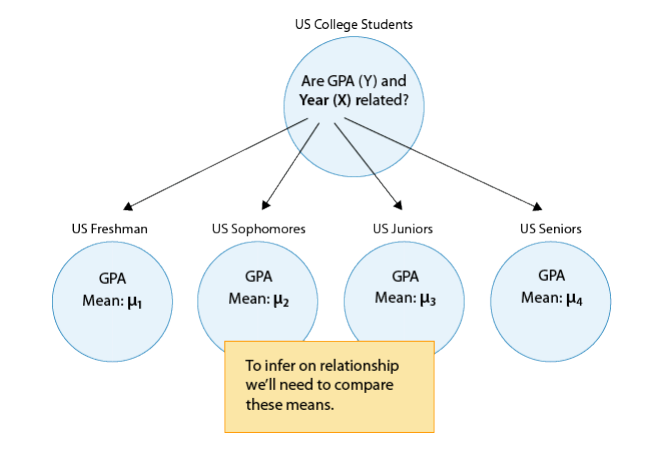
Say that our variable of interest is the GPA of college students in the United States. Since GPA is quantitative, we do inference on µ, the (population) mean GPA among all U.S. college students. We are really interested in the relationship between GPA and college year:
- X : year in college (1 = freshmen, 2 = sophomore, 3 = junior, 4 = senior)
- Y : GPA
In other words, we want to explore whether GPA is related to year in college. The way to think about this is that the population of U.S. college students is now broken into 4 subpopulations: freshmen, sophomores, juniors, and seniors. Within each of these four groups, we are interested in the GPA.
The inference must therefore involve the 4 sub-population means:
- µ1 : mean GPA among freshmen in the United States
- µ2 : mean GPA among sophomores in the United States
- µ3 : mean GPA among juniors in the United States
- µ4 : mean GPA among seniors in the United States
It makes sense that the inference about the relationship between year and GPA has to be based on some kind of comparison of these four means. If we infer that these four means are not all equal (i.e., that there are some differences in GPA across years in college) then that’s equivalent to saying GPA is related to year in college. Let’s summarize this example with a figure:
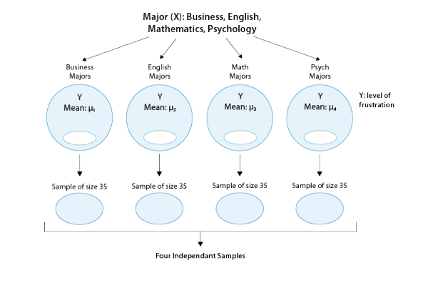
In general, then, making inferences about the relationship between X and Y in Case C→Q boils down to comparing the means of Y in the sub-populations, which are created by the categories defined in X (say k categories). The following figure summarizes this:

The inferential method for comparing means is called Analysis of Variance (abbreviated as ANOVA), and the test associated with this method is called the ANOVA F-test. We will first present our leading example, and then introduce the ANOVA F-test by going through its 4 steps, illustrating each one using the example.
Is “academic frustration” related to major?
A college dean believes that students with different majors may experience different levels of academic frustration. Random samples of size 35 of Business, English, Mathematics, and Psychology majors are asked to rate their level of academic frustration on a scale of 1 (lowest) to 20 (highest)
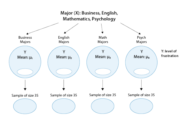
The figure highlights that examining the relationship between major (X) and frustration level (Y) amounts to comparing the mean frustration levels (µ1,µ2,µ3,µ4) among the four majors defined by X.
The Anova F-Test
Now that we understand in what kind of situations ANOVA is used, we are ready to learn how it works.
Stating the Hypotheses
The null hypothesis claims that there is no relationship between X and Y. Since the relationship is examined by comparing µ1,µ2,µ3,…µk (the means of Y in the populations defined by the values of X), no relationship would mean that all the means are equal. Therefore the null hypothesis of the F-test is: H0:µ1=µ2=…=µk.
As we mentioned earlier, here we have just one alternative hypothesis, which claims that there is a relationship between X and Y. In terms of the means µ1,µ2,µ3,…,µk, it simply says the opposite of the alternative, that not all the means are equal, and we simply write: Ha: not all the µ′s are equal.
Recall our “Is academic frustration related to major?” example:
The correct hypotheses for our example are:
- H0: µ1=µ2=µ3=µ4
- HA: Not all µi’s are the same
Note that there are many ways for µ1,µ2,µ3,µ4 not to be all equal, and µ1≠µ2≠µ3≠µ4 is just one of them. Another way could be µ1=µ2=µ3≠µ4 or µ1=µ2≠µ3=µ4. The alternative of the ANOVA F-test simply states that not all of the means are equal and is not specific about the way in which they are different.
The Idea Behind the ANOVA F-Test
Let’s think about how we would go about testing whether the population means µ1,µ2,µ3,µ4 are equal. It seems as if the best we could do is to calculate their point estimates—the sample mean in each of our 4 samples (denote them by ȳ1,ȳ2,ȳ3,ȳ4), and see how far apart these sample means are, or, in other words, measure the variation between the sample means. If we find that the four sample means are not all close together, we’ll say that we have evidence against Ho, and otherwise, if they are close together, we’ll say that we do not have evidence against Ho. This seems quite simple, but is this enough? Let’s see.
It turns out that:
- The sample mean frustration score of the 35 business majors is: ȳ1 = 7.3
- The sample mean frustration score of the 35 English majors is: ȳ2= 1.8
- The sample mean frustration score of the 35 math majors is: ȳ3= 3.2
- The sample mean frustration score of the 35 psychology majors is: ȳ4= 4.0
Below we present two possible scenarios for our example. In both cases, we construct side-by-side box plots (showing the distribution of the data including the range, lowest and highest values, the median, mean, etc.) for each of the four groups on frustration level. Scenario #1 and Scenario #2 both show data for four groups with the sample means 7.3, 11.8, 13.2, and 14.0 (means indicated with red marks).
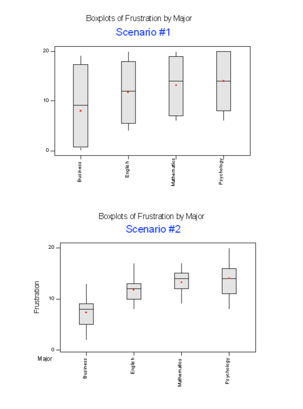
The important difference between the two scenarios is that the first represents data with a large amount of variation within each of the four groups; the second represents data with a small amount of variation within each of the four groups.
Scenario 1, because of the large amount of spread within the groups, shows box plots with plenty of overlap. One could imagine the data arising from 4 random samples taken from 4 populations, all having the same mean of about 11 or 12. The first group of values may have been a bit on the low side, and the other three a bit on the high side, but such differences could conceivably have come about by chance. This would be the case if the null hypothesis, claiming equal population means, were true. Scenario 2, because of the small amount of spread within the groups, shows boxplots with very little overlap. It would be very hard to believe that we are sampling from four groups that have equal population means. This would be the case if the null hypothesis, claiming equal population means, were false.
Thus, in the language of hypothesis tests, we would say that if the data were configured as they are in scenario 1, we would not reject the null hypothesis that population mean frustration levels were equal for the four majors. If the data were configured as they are in scenario 2, we would reject the null hypothesis, and we would conclude that mean frustration levels differ depending on major.
Let’s summarize what we learned from this. The question we need to answer is: Are the differences among the sample means ( ȳ’s) due to true differences among the µ’s (alternative hypothesis), or merely due to sampling variability (null hypothesis)?
In order to answer this question using our data, we obviously need to look at the variation among the sample means, but this alone is not enough. We need to look at the variation among the sample means relative to the variation within the groups. In other words, we need to look at the quantity:
- Variation among sample means / Variation within groups
which measures to what extent the difference among the sampled groups’ means dominates over the usual variation within the sampled groups (which reflects differences in individuals that are typical in random samples).
When the variation within groups is large (like in scenario 1), the variation (differences) among the sample means could become negligible and the data provide very little evidence against Ho.When the variation within groups is small (like in scenario 2), the variation among the sample means dominates over it, and the data have stronger evidence against Ho.
Looking at this ratio of variations is the idea behind the comparison of means; hence the name analysis of variance (ANOVA).
Did I Get This?
Suppose we are investigating interview scores for an executive level position where applicants are rated from 0 (not at all qualified) to 50 (extremely qualified). We want to investigate the effectiveness of 3 interview training programs (which we will denote — program 1, program 2, and program 3. Ultimately we would like to know whether there is an association between training program and interview scores. That is, we would like to test the hypothesis:
- H0: µ1=µ2=µ3
- HA: Not all µi’s are the same
The following are two possible scenarios of the data (note in both scenarios the sample means are 25, 30, and 35).
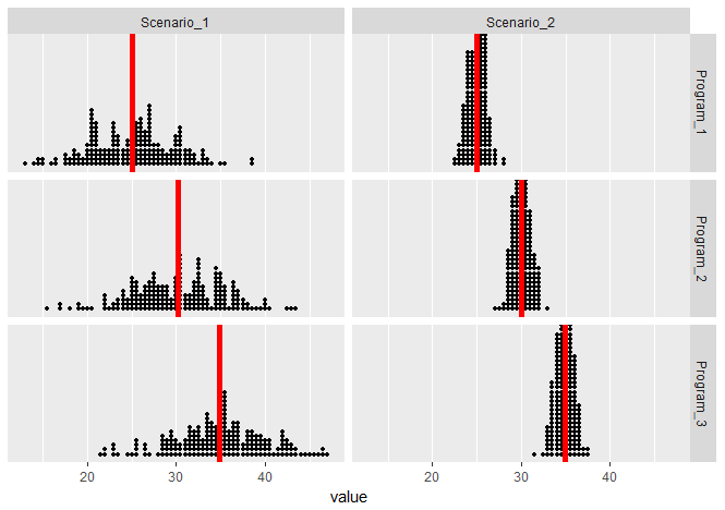
In both scenarios (since the means are the same), we have the same between group variation. But these scenarios vary greatly on their within group variation — notice that the within group variation is visibly smaller in Scenario 2 than it is in Scenario 1. Both scenarios seem to visually imply there is a relationship between Program and Interview Score, but the evidence in Scenario 2 is more compelling.
Finding the P-Value
The p-value of the ANOVA F-test is the probability of getting an F statistic as large as we got (or even larger) had H0:µ1=µ2=…=µk been true. In other words, it tells us how surprising it is to find data like those observed, assuming that there is no difference among the population means µ1, µ2, …,µk.
Returning back to our example of Academic Frustration and Major, we can obtain the following output using R, SAS, or STATA (there should be only small variations between them):
| Df | Sum Sq. | Mean Sq. | F-value | P-value | |
| Major | 3 | 939.85 | 313.28 | 46.601 | <2.2e-16 |
| Residuals | 136 | 914.29 | 6.72 |
The p-value in this example is so small that it is essentially 0, telling us that it would be next to impossible to get data like those observed had the mean frustration level of the four majors been the same (as the null hypothesis claims).
Making Conclusions in Context
As usual, we base our conclusion on the p-value. A small p-value tells us that our data contain evidence against Ho. More specifically, a small p-value tells us that the differences between the sample means are statistically significant (unlikely to have happened by chance), and therefore we reject Ho. If the p-value is not small, the data do not provide enough evidence to reject Ho, and so we continue to believe that it may be true. A significance level (cut-off probability) of .05 can help determine what is considered a small p-value.
In our example, the p-value is extremely small (close to 0) indicating that our data provide extremely strong evidence to reject Ho. We conclude that the frustration level means of the four majors are not all the same, or, in other words, that majors are related to students’ academic frustration levels at the school where the test was conducted.
Post Hoc Tests
When testing the relationship between your explanatory (X) and response variable (Y) in the context of ANOVA, your categorical explanatory variable (X) may have more than two levels.
For example, when we examine the differences in mean GPA (Y) across different college years (X=freshman, sophomore, junior and senior) or the differences in mean frustration level (Y) by college major (X=Business, English, Mathematics, Psychology), there is just one alternative hypothesis, which claims that there is a relationship between X and Y.
In terms of the means µ1,µ2,µ3,…,µk,(ANOVA), it simply says the opposite of the alternative, that not all the means are equal.
Example:
Note that there are many ways for µ1,µ2,µ3,µ4 not to be all equal, and µ1≠µ2≠µ3≠µ4 is just one of them. Another way could be µ1=µ2=µ3≠µ4 or µ1=µ2≠µ3=µ4.
In the case where the explanatory variable (X) represents more than two groups, a significant ANOVA F test does not tell us which groups are different from the others.
To determine which groups are different from the others, we would need to perform post hoc tests. These tests, done after the ANOVA, are generally termed post hoc paired comparisons.
Post hoc paired comparisons (meaning “after the fact” or “after data collection”) must be conducted in a particular way in order to prevent excessive Type I error.
Type I error occurs when you make an incorrect decision about the null hypothesis. Specifically, this type of error is made when your p-value makes you reject the null hypothesis (H0) when it is true. In other words, your p-value is sufficiently small for you to say that there is a real association, despite the fact that the differences you see are due to chance alone. The type I error rate equals your p-value and is denoted by the Greek letter α (alpha).
Although a Type I Error rate of .05 is considered acceptable (i.e. it is acceptable that 5 times out of 100 you will reject the null hypothesis when it is true), higher Type I error rates are not considered acceptable. If you were to use the significance level of .05 across multiple paired comparisons (for example, three) with p = .05, then the p rate across all three comparisons is .05+.05+.05, or .15, yielding a 15% Type I Error rate. In other words, across the unprotected paired comparisons you will reject the null hypothesis when it is true, 15 times out of 100.
The purpose of running protected post hoc tests is that they allow you to conduct multiple paired comparisons without inflating the Type I Error rate.
For ANOVA, you can use one of several post hoc tests, each which control for Type I Error, while performing paired comparisons (Duncan Multiple Range test, Dunnett’s Multiple Comparison test, Newman-Keuls test, Scheffe’s test, Tukey’s HSD test, Fisher’s LSD test, Sidak).
Please watch the video below that corresponds to the software you are using:
Hypothesis Testing and ANOVA
-
R
-
SAS
-
Stata
-
Python
Watch Playlist from Lesson 1 through Lesson 10 (Hypothesis Testing and ANOVA)
Pre-Class Quiz
After reviewing the material above, take Quiz 7 in moodle. Please note that you have 2 attempts for this quiz and the higher grade prevails.
During Class Tasks
Mini-Assignment 5 and Project Component H (if ANOVA is appropriate for your research question).