Pre-Class Reading
There are several different types of third variables that we may need to explore when studying a research question. There are three that we will be considering in this course — Covariates, confounders, and moderators. The focus of this section will be on moderating variables, but let’s briefly describe all three types:
- A covariate is a variable that is possibly predictive of the outcome under study. Think back to your literature review: are there any variables that the research shows are strong predictors of your response variable that you’d like to incorporate into your regression model? Covariates can help you build a model that does a better job of making predictions.
- A moderator is a special type of covariate. Not only does it help us predict our outcome variable, but it also seems to effect the direction or strength of the relationship between the explanatory and response variable. The effect of a moderating variable is often characterized statistically as an interaction.
- A confounder is a variable that is linked to both the explanatory variable and the response variable. Sometimes confounders make it appear that there is an interesting relationship between your explanatory and response variable. If our relationship of interest remains unchanged after including potential confounding variables into a regression model, it can make your overall story more powerful. While you won’t be able to establish causation – it does get you closer to understanding how your variables relate to one another.
Visualizing Moderating Variables
Parental Relationships and School Detention in Middle School Students
Suppose we are interested in testing whether the strength of parental relationships (as measured by a middle school students on a scale from 1(low) to 5(high)) is related to whether a student receives a detention within the first month of school. A bivariate graph reveals the following:
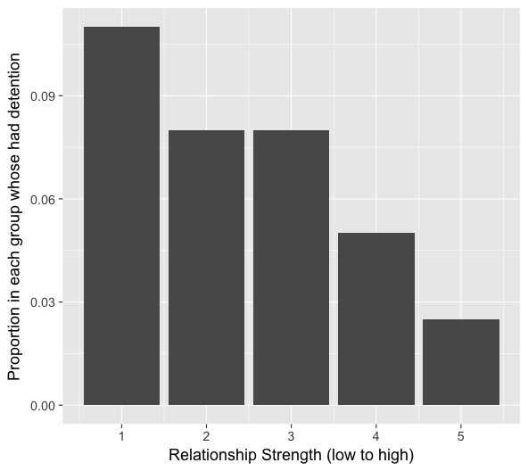
The graph above does suggest that there is an association between relationship strength and detention. Specifically, students with a stronger relationship have a lower tendency of detention. But is this relationship true for students for all grades? Let’s take a look when we break up the graph by grade level.
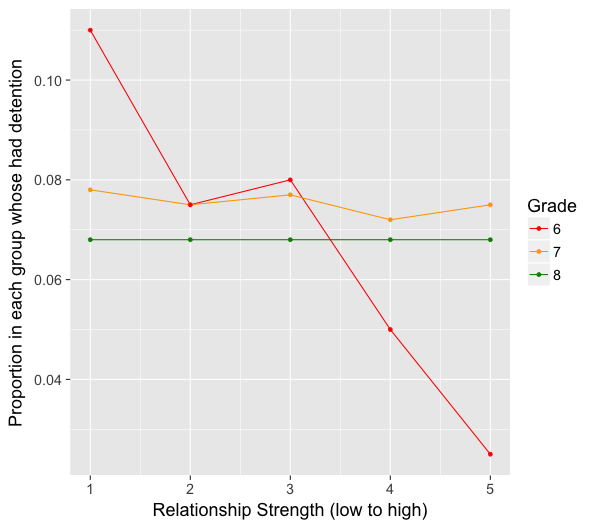
Notice that the relationship appears strong for 6th grade students in the graph above, very mild for students in 7th grade, and non-existent for students in 8th grade. Since the association between relationship strength and detention differs based on grade, it would suggest that grade is a potential moderating variable.
Interview Scores and Training Program
Suppose we are trying to study which training program (A) or (B) is more beneficial for helping job hunters during their interviews. Suppose we obtain the following graph:
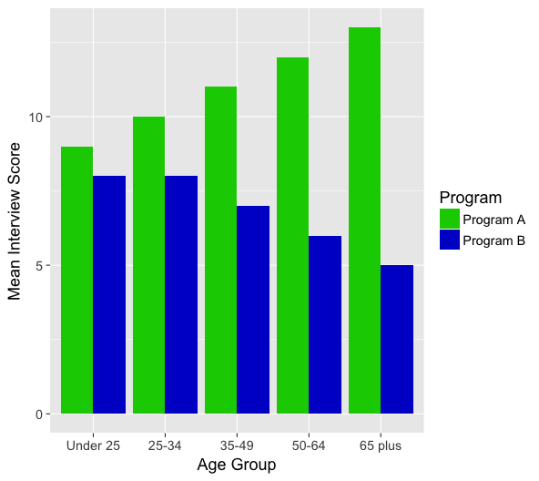
In the graph above notice that Program A is more effective than Program B across-the-board. However, Program A results in a much higher average score for the older age groups than for the younger age groups. Since the strength of the relationship between Program and Interview Score seems to vary based on age group, age group is a potential moderator.
Now suppose instead we obtain the following graph:
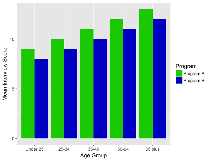
Once again, the graph above demonstrates that Program A is across-the-board more effective than Program B. In addition, the older age groups are associated with higher interview scores. Therefore, since Program A is consistently 1 unit higher than Program B within each age group, the relationship does not vary based on age. Therefore, age does NOT appear to moderate the relationship. (Age does seem like an important predictor, so can be thought of as a covariate here).
Party Affiliation and Voting
Suppose that we are looking to discover whether there is a relationship between Party Affiliation and whether someone voted. A bivariate graph shows the proportion of people who voted within each party:
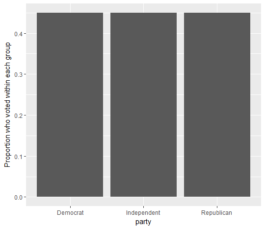
There does not appear to be a visual relationship between Political Affiliation and Voting based on the plot above since each Political Party has 45% of its members voting.
However, if we break it down by educational background, notice what might happen:
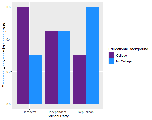
The relationship between Political Party and Voting is different based on educational background. In particular, college educated republicans are expected to vote 30% less often than college educated democrats. And non-college educated republicans are expected to vote 30% more often than non-college educated republicans. The direction of the relationship is different. This suggests that educational background is potentially a moderating variable.
How this relates to your project:
Do you think the relationship between your explanatory and response variable VARIES based on a third variable? If so, that can be a pretty interesting story to tell.
Not everyone’s project will include moderation. Take a look at your multivariate graph(s): is there a variable that meets the criteria for a potential moderator? Think about your main research question that explores the relationship between X and Y. Would it be interesting for you to explore whether the relationship was consistent across different subgroups of individuals? Would you like to state whether the relationship differed significantly? If so, it may be worthwhile for you to investigate moderation some more!
There are two approaches you can take when exploring a moderating variable.
- Analyze subsets of your data
- Regression-based approach with interaction
To help aid in the explanation of these approaches, let’s have a specific example in mind. Suppose we want to explore the relationship between years of experience in a particular job sector and salary. Our third variable of interest here is union status.
Our multivariate graph shows the following:
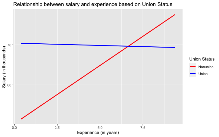
Suppose you find it really interesting that for union workers, it appears that there is no strong relationship between experience and salary, but for union workers there is a distinct positive correlation. Your next step is to find out whether statistically we can say anything about these differences.
Analyze subsets of your data
In this approach, we will study the relationship separately for union workers and non-union workers and compare our findings. This will require you to first create two subsets of your data.
Using only union workers, suppose we obtain the following regression model:
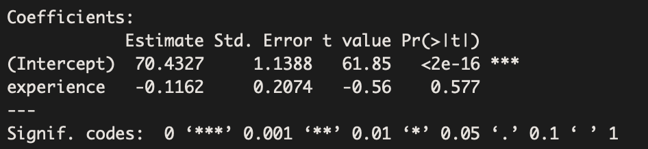
Estimated Equation: Salary = 70.4 – 0.1162(Experience)
The above statistical output tells us that there is a not a significant association between experience and salary for union workers (Beta=-0.1162, p-value=0.577).
Using only non-union workers, suppose we obtain the following regression model: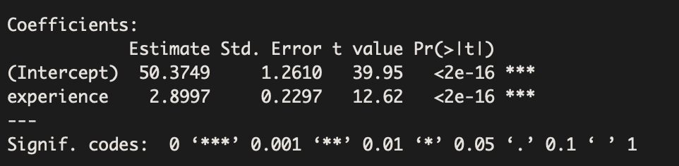
Estimated Equation: Salary = 50.4 + 2.90(Experience)
The above statistical output tells us that there is a significant association between experience and wages earned per hour for non-union workers. In particular, for each additional year of experience, the average salary is expected to increase by about 2.9 thousand dollars.
Notice that our findings about the relationship between experience and salary were quite different based on which group we were investigating. This suggests that union status does appear to moderate the relationship between experience and salary.
Regression-based approach with interaction
Including an interaction term in your model is statistically more formal, but will take a little bit more work to conceptually understand. This approach allows us to simultaneously test the relationship between experience and salary for union and non-union workers. In this approach, you use the entire data set and include an interaction term in your model.
R:
 my.lm <- lm(salary ~ experience + union + experience*union, data = myData)
summary(my.lm)
Stata:
reg salary experience i.union c.experience#i.union
SAS:
proc glm;
class union;
model salary = experience|union / solution;
run;
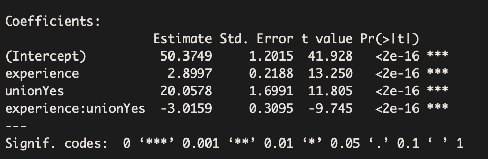
The estimated equation is: Salary = 50.37 + 2.90 (Experience) + 20.06(Union)-3.02(Experience x Union)
This one equation, allows us to model both lines.
If we plug in Union=1, we have the equation for union workers:
Salary = 50.37 + 2.90 (Experience) + 20.06(1)-3.02(Experience x 1)
Salary = 70.4 – 0.12 (Experience)
If instead we want the line for non-union workers, we would plug in Union=0:
Salary = 50.37 + 2.90 (Experience) + 20.06(0)-3.02(Experience x 0)
Salary = 50.4 + 2.90 (Experience)
Notice that these equations are nearly identical to the ones from the other method!
One of our conclusions from the output above is that experience relates to wages differently for union and non-union workers (Beta=-3.016, p-value<0.001).
Pre-Class Quiz
After reviewing the material above, take Quiz 13 in moodle. Please note that you have 2 attempts for this quiz and the higher grade prevails.
During Class Tasks
Mini-Assignment 10