Pre-Class Reading
The principles of simple linear regression lay the foundation for moving forward with more complex regression models. In this section, we will continue to consider the case where our response variable is quantitative, but will now consider the case when we have multiple explanatory variables (both categorical and quantitative).
Categorical variables as predictors
We will consider the data set ‘Pioneer’, that contains daily information on the use of a trail in the Pioneer Valley. The following information is obtained each day over a period of time:
- Average Temperature: The average temperature that day
- Season: summer, spring, fall (as a note: no data is taken over winter)
- Volume: Total number of hikers/bikers on trail
- Weekday: 1 (weekday), 0 (weekend)
- Precipitation: Measure of precipitation (in inches)
The below table shows you a small snippet of the data:
| Average Temperature | Season | Volume | Weekday | Precipitation |
|---|---|---|---|---|
| 66.5 | summer | 501 | 1 | 0.00 |
| 61.0 | summer | 419 | 1 | 0.29 |
| 63.0 | spring | 397 | 1 | 0.32 |
| 78.0 | summer | 385 | 0 | 0.00 |
| 48.0 | spring | 200 | 1 | 0.14 |
| 61.5 | spring | 375 | 1 | 0.02 |
A binary predictor variable
Let’s begin by using the variable “Weekday”, as a predictor for the volume of trail users on a given day. It is considered a binary predictor variable because it is coded as 0/1 in the dataset, where a 0 represents a weekend and a 1 represents a weekday. Our model can be obtained using the same code that was used for simple linear regression. An example of the resulting output is shown below:
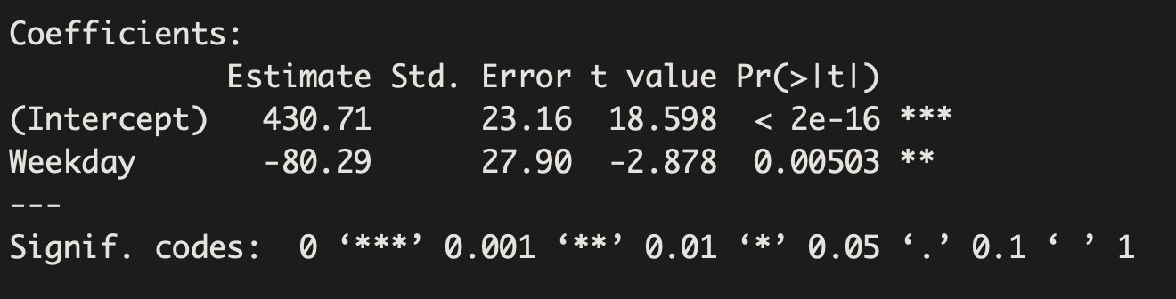
The corresponding model from the above output is:
Volume = 430.71 – 80.29 Weekday
There is strong evidence that the average volume of users on the weekend is different than the average volume of users on a weekday (Beta=-80.29, p-value=0.005). The estimate, -80.29, estimates that on a weekday the trail has 80.29 fewer users than on a weekend.
We can plug in values to make predictions. Since Weekday can only take on two values (0 for weekend and 1 for weekday), we can see our estimates below:
On a weekday (where Weekday=1), the predicted volume of users is 430.71-80.29(1)=350.42
On a weekend (where Weekday=0), the predicted volume of users is 430.71-80.29(0)=430.71
Not surprisingly, the difference between our two estimates is 80.29, which was indicated by the slope term above.
Categorical variables as predictors – beyond a binary variable
Suppose we had fit a model using a 3-level categorical variable, such as season. This regression output provides multiple rows for the season variable. Each row represents the relative difference for each level of season. However, we are missing one of the levels: fall. The missing level is called the reference level, and it represents the default level that other levels are measured against.
The equation for the regression model may be written as a model with two predictors:
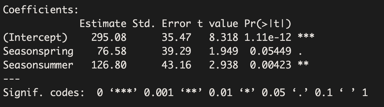
Volume = 295.08 + 76.58 Season_spring + 126.80 Season_summer
There is strong evidence that the average volume of users in summer is different than the average volume of users in fall (Beta=126.8, p-value=0.004). The estimate, 126.8, estimates that in the summer there are 126.8 more users than in the fall. There is not enough evidence to find that the average volume of users in spring is different than the average volume of users in fall (Beta=76.58, p-value=0.055). The model does not allow us to directly state whether the average volume of users in spring is significantly different than the average volume of users in summer.
Once again, we can plug values into our equation to make predictions.
If we wanted to predict the volume of users in summer: Volume = 295.08 + 76.58(0) + 126.8(1) = 421.88
If we wanted to predict the volume of users in spring: Volume = 295.08 + 76.58(1) + 126.8(0) = 371.66
If we wanted to predict the volume of users in fall: Volume = 295.08 + 76.58(0) + 126.8(0) = 295.08
Multiple Predictor Variables
Multiple linear regression can be used when we wish to examine how a collection of explanatory variables (both quantitative and categorical) helps us to predict a quantitative response variable of interest.
Example 1:
Now let’s suppose we are interested in how the dosage (in mg) of a particular drug relates to post-treatment depression scores among individuals who were diagnosed with depression. (For this example, depression is a quantitative variable ranging from 0 to 65). Our research question might therefore be: How does drug dosage relate to post-treatment depression?
We might first begin by examining the association between these two variables:
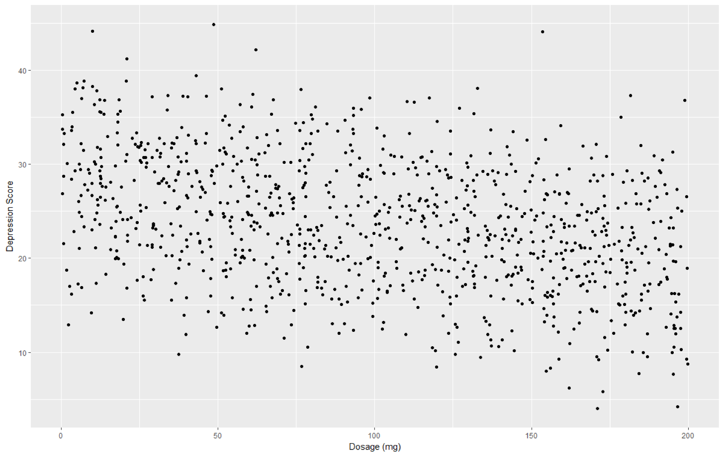
The initial model under consideration is a simple regression model since it has only a single predictor variable.
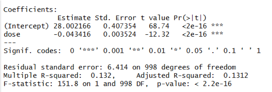
The regression model indicates that there is a significant association between dose and depression (Beta=-0.04, p < 0.001). The model predicts that for each additional 1mg of drug, the depression score is expected to be 0.04 points lower on average.
Ultimately, we may want to try to improve the accuracy of our predictions by including additional variables that may help predict depression. Suppose we believe poverty (coded 0/1) is an important predictor of depression. Let us first see whether poverty appears to be visually related to depression in addition to dosage:
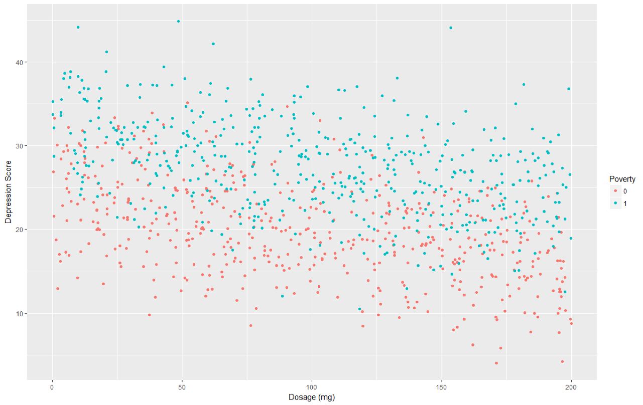
You may notice that it appears that those in poverty do appear to have slightly higher depression scores than those not in poverty, regardless of dosage.
Using multiple linear regression model to incorporate this additional explanatory variable results in the following model:
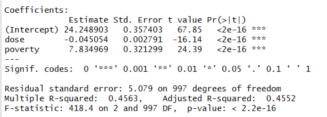
The model that is used to describe the data above is now:
Depression = 24.25 – 0.045 (Dose) + 7.835 (Poverty)
This model can be visualized as follows:
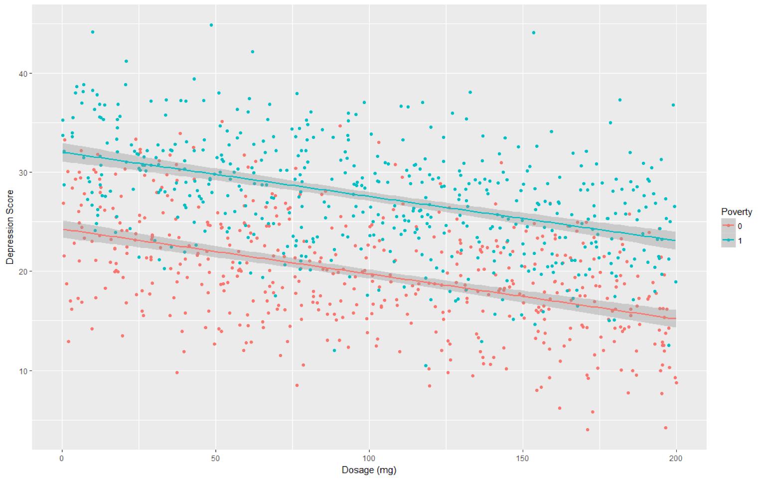
The regression model indicates that there is a significant association between dose and depression (Beta=-0.04, p < 0.001) and also between poverty and depression (Beta=7.835, p < 0.001). The model predicts that for each additional 1mg of drug, the depression score is expected to be 0.04 points lower on average when we hold poverty fixed. Additionally, the model predicts that someone in poverty has an average depression score that is 7.845 units higher than someone not in poverty when we hold dosage fixed (this can be seen graphically, as the distance between the two lines for poverty status are 7.845 units apart across the entire plot). It is important to note that the model run for this example is forcing these lines to be parallel. In this example, forcing the lines to be parallel does seem like an appropriate choice. When we do not wish to assume the lines are parallel – we may wish to consider an interaction term in our model.
Example 2:
Suppose we are interested in seeing how a training program and work experience collectively help predict job performance. Workers are randomly assigned to 1 of 3 training programs (Standard, New Option A, New Option B) and work experience is recorded in years. Job performance is a quantitative variable that ranges from 0 (low) to 40 (high).
Suppose we wish to construct a model that allows us to predict job performance based on experience and training program. The output is shown below:
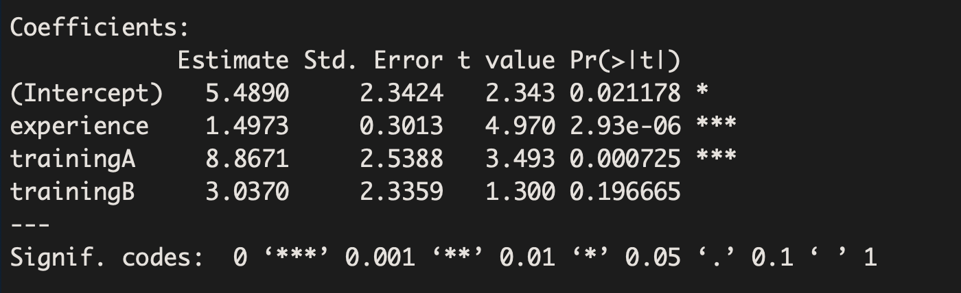
The output can be used to write out the following model:
Job Performance= 5.5 + 1.5 Experience + 8.9 TrainingA +3.0 TrainingB
This model can be visualized as follows:
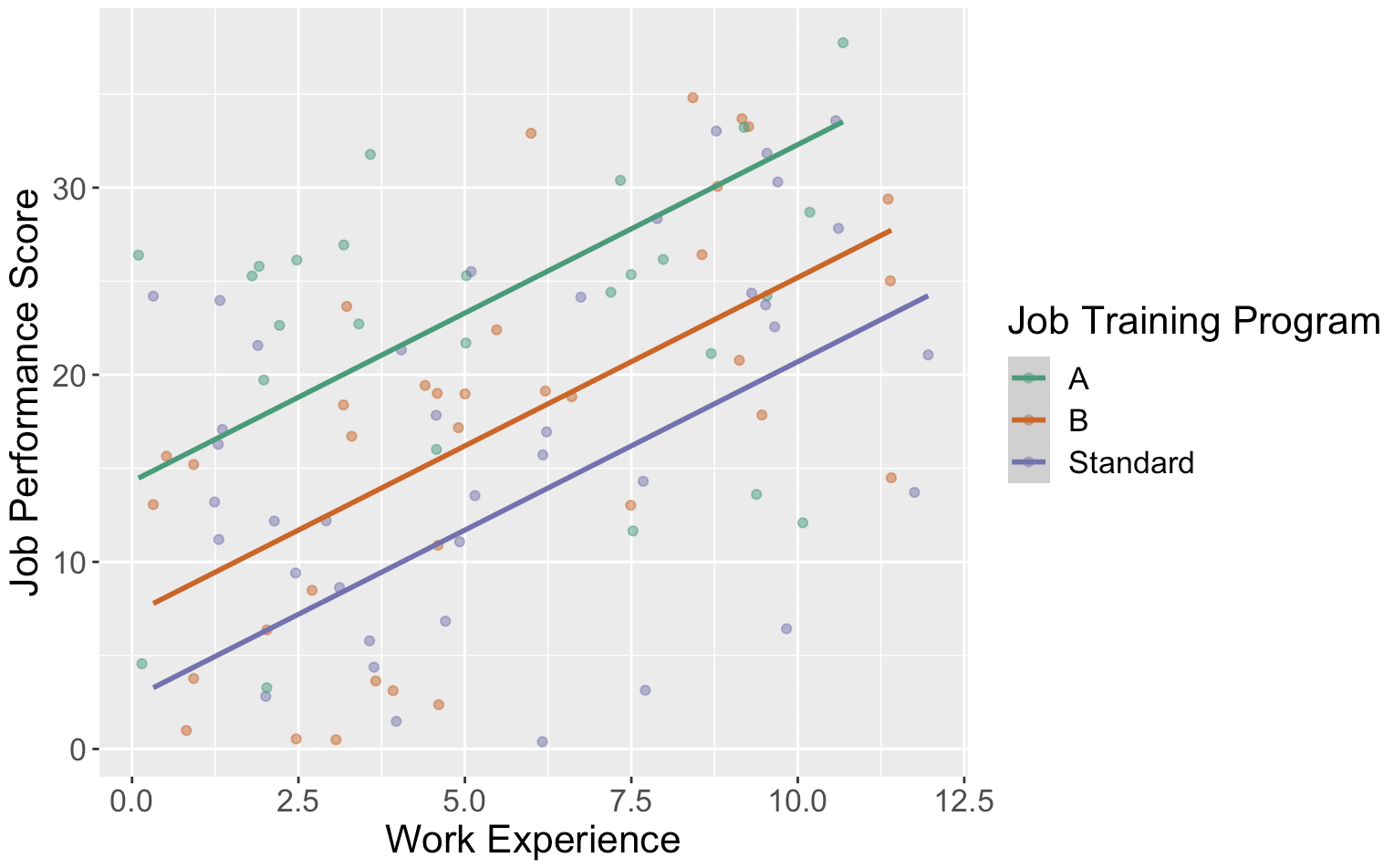
The regression model indicates that there is a significant difference in job performance between those who are assigned to Training Option A and those who are assigned to the Standard Option (Beta=8.9, p = 0.0007) when we hold work experience fixed. If you look at the variables visually, you can see that regardless of work experience, that the model is predicting those in Training Option A have an average job performance that is 8.9 units higher than those in the standard training program.
There is not sufficient evidence to suggest that Training Option B is significantly different than the Standard Option (Beta=3.0, p = 0.1967) when we hold work experience fixed.
Finally, the model suggests that work experience is a significant predictor of job performance (Beta=1.5, p-value<0.001). The model predicts that for each additional year of work experience, job performance is expected to increase on average by 1.5 points when we hold training program fixed.
The model we used is assuming that no matter what training program someone is in, we expected that each additional year of work experience is associated with the same average change in job performance.
During-Class Tasks
Work on Mini-Assignment 8 and then consider additional variables to incorporate into your project. Construct a plot or two that explore how these additional variables collectively relate to your response variable.