Pre-Class Reading
Sampling and Designing Studies
Suppose you want to determine the musical preferences of all students at your university based on a sample of students. Here are some examples of the many possible ways to pursue this problem.
Example #1:
Post a music-lovers’ survey on a university Internet bulletin board, asking students to vote for their favorite type of music.
This is an example of a volunteer sample, where individuals have selected themselves to be included. Such a sample is almost guaranteed to be biased. In general, volunteer samples tend to be comprised of individuals who have a particularly strong opinion about an issue and are looking for an opportunity to voice it. Whether the variable’s values obtained from such a sample are over- or under-stated, and to what extent, cannot be determined. As a result, data obtained from a voluntary response sample is quite useless when you think about the “Big Picture”, since the sampled individuals only provide information about themselves, and we cannot generalize to any larger group at all.
Comment: It should be mentioned that in some cases volunteer samples are the only ethical way to obtain a sample. In medical studies, for example, in which new treatments are tested, subjects must choose to participate by signing a consent form that highlights the potential risks and benefits. As we will discuss in the next module, a volunteer sample is not so problematic in a study conducted for the purpose of comparing several treatments.
Example #2:
Stand outside the Student Union, across from the Fine Arts Building, and ask students passing by to respond to a question about musical preference.
This is an example of a convenience sample, where individuals happen to be at the right time and place to suit the schedule of the researcher. Depending on what variable is being studied, it may be that a convenience sample provides a fairly representative group. However, there are often subtle reasons why the sample’s results are biased. In this case, the proximity to the Fine Arts Building might result in a disproportionate number of students favoring classical music. A convenience sample may also be susceptible to bias because certain types of individuals are more likely to be selected than others. In the extreme, some convenience samples are designed in such a way that certain individuals have no chance at all of being selected, as in the next example.
Example #3:
Ask your professors for email rosters of all the students in your classes. Randomly sample some addresses and email those students with your question about musical preference.
Here is a case where the sampling frame—list of potential individuals to be sampled—does not match the population of interest. The population of interest consists of all students at the university, whereas the sampling frame consists of only your classmates. There may be bias arising because of this discrepancy. For example, students with similar majors will tend to take the same classes as you, and their musical preferences may also be somewhat different from those of the general population of students. It is always best to have the sampling frame match the population as closely as possible.
Example #4:
Obtain a student directory with email addresses of all the university’s students and send the music poll to every 50th name on the list.
This is called systematic sampling. It may not be subject to any clear bias, but it would not be as safe as taking a random sample.
If individuals are sampled completely at random and without replacement, then each group of a given size is just as likely to be selected as all the other groups of that size. This is called a simple random sample (SRS). In contrast, a systematic sample would not allow sibling students to be selected because they have the same last name. In a simple random sample, sibling students would have just as much of a chance of both being selected as any other pair of students. Therefore, there may be subtle sources of bias in using a systematic sampling plan.
Example #5:
Obtain a student directory with email addresses of all the university’s students and send your music poll to a simple random sample of students. As long as all of the students respond, then the sample is not subject to any bias and should succeed in being representative of the population of interest.
But what if only 40% of those selected email you back with their vote?
The results of this poll would not necessarily be representative of the population because of the potential problems associated with volunteer response. Since individuals are not compelled to respond, often a relatively small subset take the trouble to participate. Volunteer response is not as problematic as a volunteer sample (presented in example 1 above), but there is still a danger that those who do respond are different from those who don’t with respect to the variable of interest. An improvement would be to follow up with a second email, asking politely for students’ cooperation. This may boost the response rate, resulting in a sample that is fairly representative of the entire population of interest, and it may be the best that you can do under the circumstances. Nonresponse is still an issue, but at least you have managed to reduce its impact on your results.
So far we’ve discussed several sampling plans and determined that a simple random sample is the only one we discussed that is not subject to any bias.
A simple random sample is the easiest way to base a selection on randomness. There are other, more sophisticated, sampling techniques that utilize randomness that are often preferable in real-life circumstances. Any plan that relies on random selection is called a probability sampling plan (or technique). The following three probability sampling plans are among the most commonly used:
- Simple Random Sampling—Simple random sampling, as the name suggests, is the simplest probability sampling plan. It is equivalent to “selecting names out of a hat”. Each individual has the same chance of being selected.
- Cluster Sampling—Cluster sampling is used when our population is naturally divided into groups (which we call clusters). For example, all the students in a university are divided into majors; all the nurses in a certain city are divided into hospitals; all registered voters are divided into precincts (election districts). In cluster sampling, we take a random sample of clusters, and use all the individuals within the selected clusters as our sample. For example, in order to get a sample of highschool seniors from a certain city, you choose 3 high schools at random from among all the high schools in that city and use all the high school seniors in the three selected high schools as your sample.
- Stratified Sampling—Stratified sampling is used when our population is naturally divided into subpopulations, which we call strata (singular: stratum). For example, all the students in a certain college are divided by gender or by year in college; all the registered voters in a certain city are divided by race. In stratified sampling, we choose a simple random sample from each stratum, and our sample consists of all these simple random samples put together. For example, in order to get a random sample of high-school seniors from a certain city, we choose a random sample of 25 seniors from each of the high schools in that city. Our sample consists of all these samples put together.
Each of those probability sampling plans, if applied correctly, are not subject to any bias and thus produce samples that represent well the population from which they were drawn.
Comment: Cluster vs. Stratified Students sometimes get confused about the difference between cluster sampling and stratified sampling. Even though both methods start out with the population somehow divided into groups, the two methods are very different. In cluster sampling, we take a random sample of whole groups of individuals, while in stratified sampling we take a simple random sample from each group. For example, say we want to conduct a study on the sleeping habits of undergraduate students at a certain university and need to obtain a sample. The students are naturally divided by majors, and let’s say that in this university there are 40 different majors. In cluster sampling, we would randomly choose, say, 5 majors (groups) out of the 40 and use all the students in these five majors as our sample. In stratified sampling, we would obtain a random sample of, say, 10 students from each of the 40 majors (groups) and use the 400 chosen students as the sample. Clearly in this example, stratified sampling is much better since the major of the student might have an effect on the student’s sleeping habits, and so we would like to make sure that we have representatives from all the different majors. We’ll stress this point again following the example and activity.
Suppose you would like to study the job satisfaction of hospital nurses in a certain city based on a sample. Besides taking a simple random sample, here are two additional ways to obtain such a sample.
1. Suppose that the city has 10 hospitals. Choose one of the 10 hospitals at random and interview all the nurses in that hospital regarding their job satisfaction. This is an example of cluster sampling, in which the hospitals are the clusters.
2. Choose a random sample of 50 nurses from each of the 10 hospitals and interview these 50 * 10 = 500 regarding their job satisfaction. This is an example of stratified sampling, in which each hospital is a stratum.
Cluster or Stratified—Which One is Better? Let’s go back and revisit the job satisfaction of hospital nurses example and discuss the pros and cons of the two sampling plans that are presented. Certainly, it will be much easier to conduct the study using the cluster sample because all interviews are conducted in one hospital as opposed to the stratified sample, in which the interviews need to be conducted in 10 different hospitals. However, the hospital that a nurse works in probably has a direct impact on his/her job satisfaction, and, in that sense, getting data from just one hospital might provide biased results. In this case, it will be very important to have representation from all the city hospitals, and therefore the stratified sample is definitely preferable. On the other hand, say that, instead of job satisfaction, our study focuses on the age or weight of hospital nurses.
In this case, it is probably not as crucial to get representation from the different hospitals, and therefore the more easily obtained cluster sample might be preferable.
Designing Studies
Obviously, sampling is not done for its own sake. After this first stage in the data production process is completed, we come to the second stage, that of gaining information about the variables of interest from the sampled individuals. In this module we’ll discuss three study designs; each design enables you to determine the values of the variables in a different way. You can:
- Carry out an observational study, in which values of the variable or variables of interest are recorded as they naturally occur. There is no interference by the researchers who conduct the study.
- Take a sample survey, which is a particular type of observational study in which individuals report variables’ values themselves, frequently by giving their opinions. –
- Perform an experiment. Instead of assessing the values of the variables as they naturally occur, the researchers interfere, and they are the ones who assign the values of the explanatory variable to the individuals. The researchers “take control” of the values of the explanatory variable because they want to see how changes in the value of the explanatory variable affect the response variable. (Note: By nature, any experiment involves at least two variables.)
The type of design used and the details of the design are crucial because they will determine what kind of conclusions we may draw from the results. In particular, when studying relationships in the Exploratory Data Analysis unit, we stressed that an association between two variables does not guarantee that a causal relationship exists. In this module, we will explore how the details of a study design play a crucial role in determining our ability to establish evidence of causation.
Identifying Study Design
Because each type of study design has its own advantages and trouble spots, it is important to begin by determining what type of study we are dealing with. The following example helps to illustrate how we can distinguish among the three basic types of design mentioned in the introduction—observational studies, sample surveys, and experiments.
Suppose researchers want to determine whether people tend to snack more while they watch television. In other words, the researchers would like to explore the relationship between the explanatory variable “TV” (a categorical variable that takes the values “on’” and “not on”) and the response variable “snack consumption”.
Identify each of the following designs as being an observational study, a sample survey, or an experiment.
- EX1: Recruit participants for a study. While they are presumably waiting to be interviewed, half of the individuals sit in a waiting room with snacks available and a TV on. The other half sit in a waiting room with snacks available and no TV, just magazines. Researchers determine whether people consume more snacks in the TV setting.
This is an experiment, because the researchers take control of the explanatory variable of interest (TV on or not) by assigning each individual to either watch TV or not and determine the effect that has on the response variable of interest (snack consumption).
- EX2: Recruit participants for a study. Give them journals to record hour by hour their activities the following day, including when they watch TV and when they consume snacks. Determine if snack consumption is higher during TV times.
This is an observational study, because the participants themselves determine whether or not to watch TV. There is no attempt on the researchers’ part to interfere.
- EX3: Recruit participants for a study. Ask them to recall, for each hour of the previous day, whether they were watching TV and what snacks they consumed each hour. Determine whether snack consumption was higher during the TV times.
This is also an observational study; again, it was the participants themselves who decided whether or not to watch TV. Do you see the difference between 2 and 3? See the comment below.
- EX4: Poll a sample of individuals with the following question: “While watching TV, do you tend to snack: (a) less than usual; (b) more than or usual; or (c) the same amount as usual?”
This is a sample survey, because the individuals self-assess the relationship between TV watching and snacking.
Comment: Notice that, in Example 2, the values of the variables of interest (TV watching and snack consumption) are recorded forward in time. Such observational studies are called prospective. In contrast, in EX3, the values of the variables of interest are recorded backward in time. This is called a retrospective observational study.
Experiments vs. Observational Studies
Before assessing the effectiveness of observational studies and experiments for producing evidence of a causal relationship between two variables, we will illustrate the essential differences between these two designs.
Every day, a huge number of people are engaged in a struggle whose outcome could literally affect the length and quality of their life: they are trying to quit smoking. Just the array of techniques, products, and promises available shows that quitting is not easy, nor is its success guaranteed. Researchers would like to determine which of the following is the best method:
- Drugs that alleviate nicotine addiction.
- Therapy that trains smokers to quit.
- A combination of drugs and therapy.
- Neither form of intervention (quitting “cold turkey”).
The explanatory variable is the method (1, 2, 3 or 4) , while the response variable is eventual success or failure in quitting. In an observational study, values of the explanatory variable occur naturally. In this case, this means that the participants themselves choose a method of trying to quit smoking. In an experiment, researchers assign the values of the explanatory variable. In other words, they tell people what method to use. Let us consider how we might compare the four techniques, via either an observational study or an experiment.
An observational study of the relationship between these two variables requires us to collect a representative sample from the population of smokers who are beginning to try to quit. We can imagine that a substantial proportion of that population is trying one of the four above methods. In order to obtain a representative sample, we might use a nationwide telephone survey to identify 1,000 smokers who are just beginning to quit smoking. We record which of the four methods the smokers use. One year later, we contact the same 1,000 individuals and determine whether they succeeded.
In an experiment, we again collect a representative sample from the population of smokers who are just now trying to quit by using a nationwide telephone survey of 1,000 individuals. This time, however, we divide the sample into 4 groups of 250 and assign each group to use one of the four methods to quit. One year later, we contact the same 1,000 individuals and determine whose attempts succeeded while using our designated method.
Both the observational study and the experiment begin with a random sample from the population of smokers just now beginning to quit. In both cases, the individuals in the sample can be divided into categories based on the values of the explanatory variable: method used to quit. The response variable is success or failure after one year. Finally, in both cases, we would assess the relationship between the variables by comparing the proportions of success of the individuals using each method, using a two-way table and conditional percentages.
The only difference between the two methods is the way the sample is divided into categories for the explanatory variable (method). In the observational study, individuals are divided based upon the method by which they choose to quit smoking. The researcher does not assign the values of the explanatory variable, but rather records them as they naturally occur. In the experiment, the researcher deliberately assigns one of the four methods to each individual in the sample. The researcher intervenes by controlling the explanatory variable and then assesses its relationship with the response variable.
Now that we have outlined two possible study designs, let’s return to the original question: which of the four methods for quitting smoking is most successful? Suppose the study’s results indicate that individuals who try to quit with the combination drug/therapy method have the highest rate of success, and those who try to quit with neither form of intervention have the lowest rate of success, as illustrated in the hypothetical two-way table below:
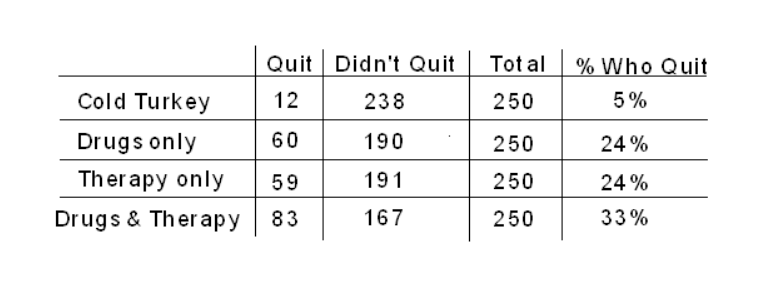
Can we conclude that using the combination drugs and therapy method caused the smokers to quit most successfully? Which type of design was implemented will play an important role in the answer to this question.
Linear Regression
So far we’ve used the scatterplot to describe the relationship between two quantitative variables, and, in the special case of a linear relationship, we have supplemented the scatterplot with the correlation (r). The correlation, however, doesn’t fully characterize the linear relationship between two quantitative variables—it only measures the strength and direction. We often want to describe more precisely how one variable changes with the other (by “more precisely,” we mean more than just the direction) or predict the value of the response variable for a given value of the explanatory variable. In order to be able to do that, we need to summarize the linear relationship with a line that best fits the linear pattern of the data. In the remainder of this section, we will introduce a way to find such a line, learn how to interpret it, and use it (cautiously) to make predictions. Again, let’s start with a motivating example: Earlier, we examined the linear relationship between the age of a driver and the maximum distance at which a highway sign was legible, using both a scatterplot and the correlation coefficient. Suppose a government agency wanted to predict the maximum distance at which the sign would be legible for 60-year old drivers and thus make sure that the sign could be used safely and effectively.
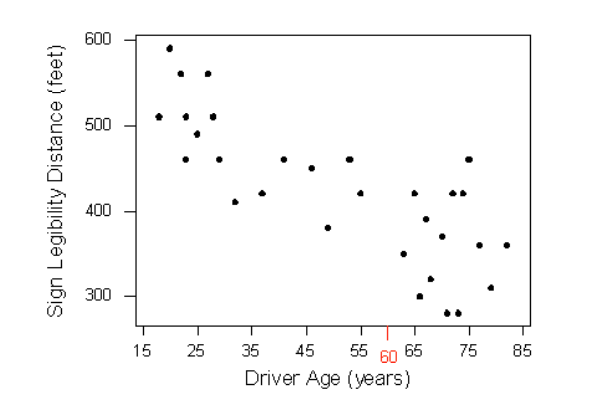
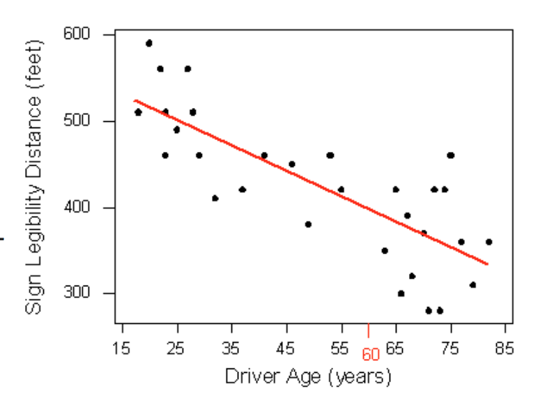
How can we make this prediction at which a sign is legible? The age for which an agency wishes to predict the legibility distance, 60, is marked in red. It would be useful if we could find a line (such as the one that is presented on the scatterplot below) that represents the general pattern of the data.
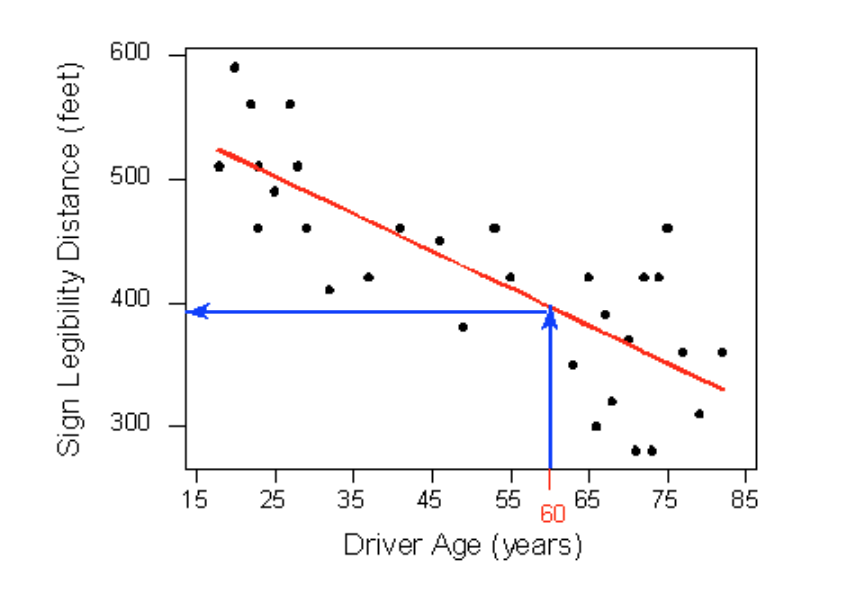
Then we would simply use this line to find the distance that corre- sponds to an age of 60 like this:
and predict that 60-year-old drivers could see the sign from a distance of just under 400 feet.
To understand how such a line is chosen, consider the following very simplified version of the age-distance example (we left just 6 of the drivers on the scatterplot):
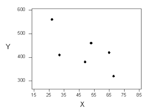
There are many lines that look like they would be good candidates to be the line that best fits the data:
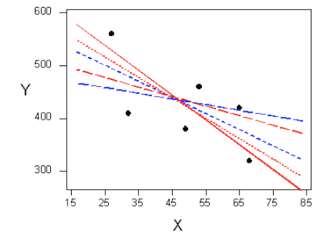
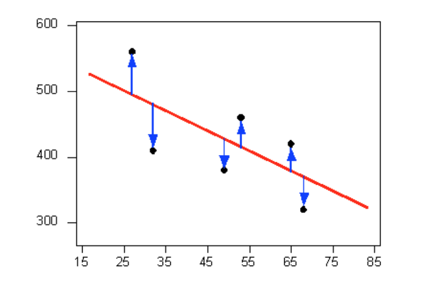
It is doubtful that everyone would select the same line in the plot above. We need to agree on what we mean by “best fits the data”; in other words, we need to agree on a criterion by which we would select this line. We want the line we choose to be close to the data points. In other words, whatever criterion we choose, it must take into account the vertical deviations of the data points from the line, which are marked with blue arrows in the plot below:
The most commonly used criterion is called the least squares criterion. This criterion says that among all the lines that look good on your data, choose the one that has the smallest sum of squared vertical deviations. Visually, each squared deviation is represented by the area of one of the squares in the plot below. Therefore, we are looking for the line that will have the smallest total yellow area.
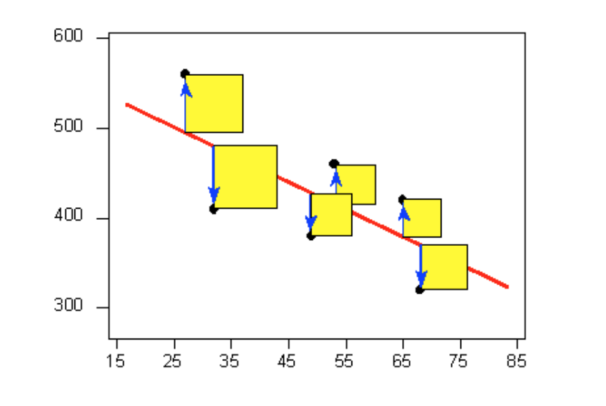
This line is called the least-squares regression line, and, as we’ll see, it fits the linear pattern of the data very well. For the remainder of this lesson, you’ll need to feel comfortable with the algebra of a straight line. In particular, you’ll need to be familiar with the slope and the intercept in the equation of a line and their interpretation. Like any other line, the equation of the least-squares regression line for summarizing the linear relationship between the response variable (Y) and the explanatory variable (X) has the form: Y=β0+β1X.
We will be using our statistical software in order to compute this least squares regression line. Once we have our estimated regression line, predictions become quite straightforward.
Let’s go back now to our motivating example, in which we wanted to predict the maximum distance at which a sign is legible for a 60-year-old. The least squares regression line, can be found to be:
Distance = 576 + (- 3 * Age)
We plug Age = 60 into the regression line equation, to find that:
Predicted distance = 576 + (- 3 * 60) = 396
396 feet is our best prediction for the maximum distance at which a sign is legible for a 60-year-old.
In addition, the slope tells us how we expect the predicted maximum distance to change as someone grows older. In particular, for each additional year of age, the maximum distance at which a sign is legible reduces by 3ft on average.
Linear Regression – Statistical Output
Example
Suppose we want to look at the relationship between mpg of a vehicle and the corresponding weight of a vehicle. Ultimately we would like to see whether weight can help us predict mpg of a car (Weight is in thousands of pounds).
To begin, we may wish to investigate a bivariate scatterplot of the relationship between the two variables. Weight is measured in thousands of pounds.
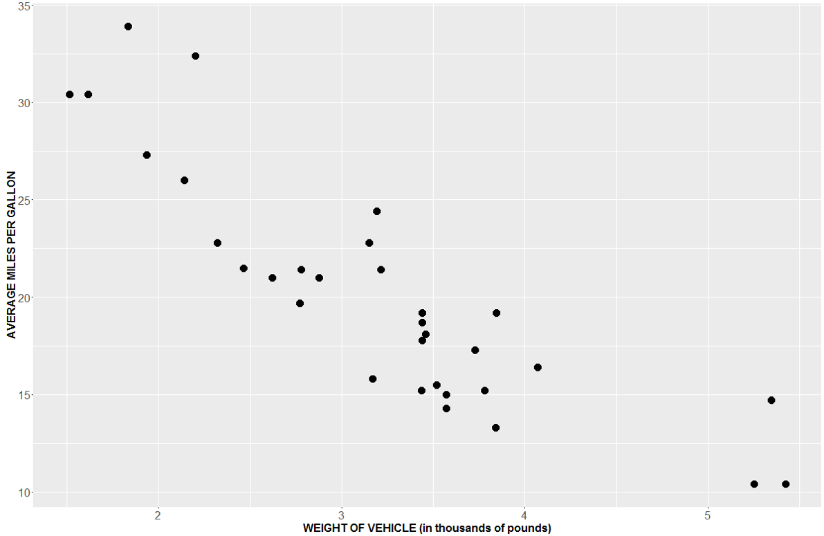
There does appear to be a visibly strong negative linear relationship between the two variables. Our next question might be: Is there a statistically significant linear relationship between weight and mpg? One way to test this is with the Pearson Correlation test. The Pearson Correlation test reveals that there is a significant linear relationship between mpg and weight (r=-0.87, p-value<0.001).
Another way to test this is with Simple Linear Regression. That is, we will aim to find the line that fits the data “best”.
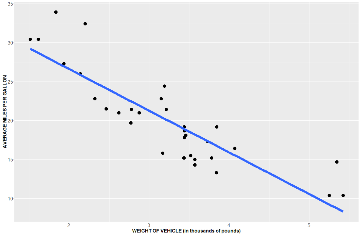
If the slope is different than 0, then it tells us that our X and Y variables have a linear relationship. Here, you can see a very distinct negative slope, but is the slope significantly different than 0?
Our hypothesis in regression is typically:
H0: There is no linear relationship between X and Y, i.e. the slope (B1) is equal to 0
HA: There is a linear relationship between X and Y, i.e. the slope (B1) is not equal to 0
Using our statistical software, we can test this hypothesis and obtain a least squares regression line. Sample output is shown below:
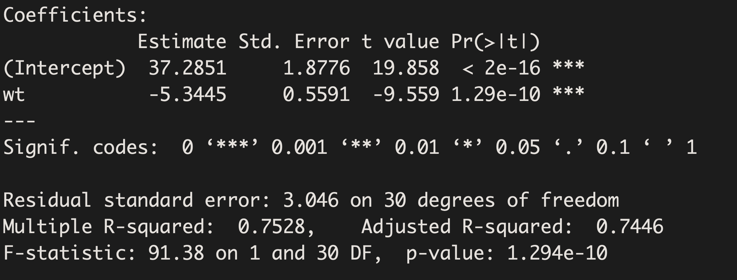
R:
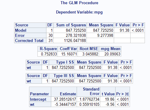
SAS:
Stata:
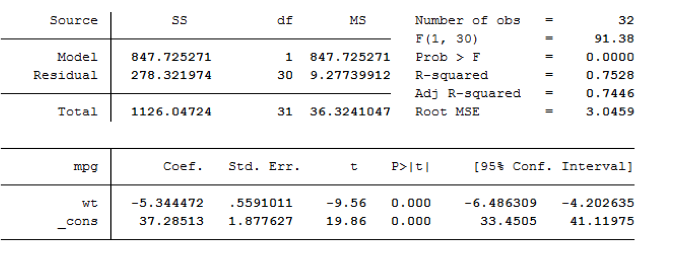
Our least squares regression equation can be found by looking at our estimates/coefficients.

For each additional unit increase in X (here, that is a 1,000 pound increase), we expect MPG to decrease on average by 5.3 mpg. This decrease is deemed significantly different from 0 (t=-9.56, p-value<0.001).
These equations can also be used to make predictions. That is, if a car weighs 2,500 pounds, how much would we predict it’s mpg to be?
37.3 – 5.3 (2.5)=24 mpg
Generally, a y-intercept term can tell us the predicted value of our response variable when our explanatory variable is 0. The intercept term in this example, 37.3, tells us the estimated predicted mpg for a car weighing 0 pounds. Here this prediction is nonsense since we would never truly want to estimate the mpg of a non-existent vehicle and it is heavily extrapolated from our model.
During-Class Tasks
Mini-Assignment 7